identifying feature points in an image

Techniques used in this article for identifying feature points in an image are inspired by SIFT algorithm.

What is a feature?

A feature is typically defined as an “interesting” part of an image, and features are used as a starting point for many computer vision algorithms.

What is SIFT algorithm?

SIFT(Scale-Invariant Feature Transform) is a feature detection algorithm in computer vision to detect and describe local features in images. It was published by David Lowe in 1999. This algorithm uses `Difference of Gaussians` (DoG) in scale space criterion.

DoG is used to identify the edges.

How? = By subtraction of one Gaussian blurred version of an original image from another, less blurred version of the original.

What is difference of gaussian? [1]

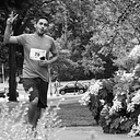
Image used for identifying features

Old house from a city, called Veere, in the province of Zeeland

Let’s take a look at the steps used in our technique:

1. Convert the image into grayscale (because the color is complex and creates more noise).
2. Creating twelve Gaussian smoothing Kernels (filter used for blurring the images). Smoothing kernels increase in intensity. These blurred images will later be used for edge detection.

few result images after smoothing (to show all 12 images might not be interesting):

smoothened to a bit lower scale

smoothened to a higher scale

3. Calculate the difference of gaussian (DoG).

DoG between two layers at lower scales (5 and 6)

DoG between two layers at higher scales (10 and 11)

4. Find key points by thresholding all 11 DoGs from above step using some threshold value. The resulting images will have three co-ordinates (x,y,𝜎).

x,y = spatial and 𝜎 = scale at which the key points were detected

5. Derivatives of all scale-space images are calculated using some kernel (like dx = (1,0,-1) and dy = (1 0 -1)T). Kernel is a small matrix used to apply effects.

few results:

gx images (notice that the lines are in x direction)

gy images (notice that the lines are in y direction)

6. Calculate gradient length and direction around the grid of points (let's consider 7x7), sampled around each key-point. In order to do so, we will be using the scale determined in step 4 and the correct gradient images from step 5. Further, we calculate a Gaussian weighting function for each grid point.

7. We find the orientation of the key-point based on the 36-bin orientation histogram vector. In other words, the key point with a max value of gradient direct will be the orientation of the key-point.

8. Draw all key-points, with radius in accordance to the scale at which they were found.

references:

[1] https://www.researchgate.net/figure/The-process-of-local-extrema-detection-based-on-Difference-of-Gaussian-DoG_fig7_273897393

[2] https://opencv-python-tutroals.readthedocs.io/en/latest/py_tutorials/py_feature2d/py_sift_intro/py_sift_intro.html